_ Alexander Jungbluth, junior economist, MIWI Institute for Market Integration and Economic Policy. Munich, 27 May 2022.
1. Introduction
After the financial crisis that began in 2008 and a gradual recovery in the global economic situation, the 2010s can be seen as very good economically until the corona pandemic in early 2020. At the beginning of 2010, the gross domestic product (GDP) in Germany was around 2,564.4 billion euros, at the beginning of 2020 it was around 3,473.4 billion euros. [1] This corresponds to an average growth in economic output of 3.08% per year.
A positive economic development is generally accompanied by an improvement in the fiscal situation in the form of higher tax revenues and a more favorable debt development. Total tax revenue increased from around 530.6 billion euros at the beginning of 2010 to around 799.3 billion euros at the beginning of 2020. [2] The average annual growth of 4.18% is well above the value of economic growth. The change in debt, based on all regional authorities, was only able to change sign in the mid-2010s. While the debt increased between 2010 and 2014, it then fell from a value of 2,043.9 billion euros to a value of 1,899.06 billion euros at the beginning of 2020. [3]
The subject of the following investigation is to determine who has benefited most from the indirect consequences of the boom in relation to the development of debt.
2. Debt development
With regard to the development of debt, an examination of the German federal government, all of the federal states and all of the municipalities is presented first, and in a next step a differentiation of the individual federal states is observed.
2.1. Overall consideration
The mere statement that there was a reduction in public budget debt from around the mid-2010s requires further analysis. According to the Federal Ministry of Finance, the debt developed as follows:
Table 1. German public sector debt (2010-2019, in mln. euros)
| 2010 | 2011 | 2012 | 2013 | 2014 | 2015 | 2016 | 2017 | 2018 | 2019 | |
| Total public budget | 2.011.677 | 2.025.438 | 2.068.289 | 2.043.344 | 2.043.918 | 2.020.704 | 2.009.310 | 1.969.104 | 1.915.767 | 1.898.762 |
| Federal government (core and extra budgets) | 1.287.460 | 1.279.583 | 1.287.517 | 1.282.683 | 1.289.854 | 1.262.769 | 1.257.065 | 1.242.547 | 1.213.302 | 1.188.581 |
| Federal states (core and extra budgets) | 600.110 | 615.399 | 644.929 | 624.915 | 614.055 | 613.202 | 608.731 | 586.394 | 570.525 | 578.762 |
| Municipalities (core and extra budgets) | 123.569 | 129.633 | 135.178 | 135.116 | 139.448 | 144.245 | 143.079 | 139.725 | 131.813 | 131.362 |
Source: [4]; MIWI Institute.
It is already evident that a debt reduction of the general public debt doesn’t occur until 2015, and that the federal government could reduce its level of debt as soon as the boom began and in the years that followed. Both the federal states and the municipalities took on new debts in their net position in the first few years. Debt reduction then began in the states from 2013, and in the municipalities only from 2016 (see Figure 1).
This development can be clearly seen from the polynomial trend lines of the three curves. While the federal and state governments show an almost time-delayed parallel course, the course of the curve for the municipalities is opposite in the first few years and only later adapts to that of the federal and state governments.
Between 2016 and 2019, there then was a reduction in the debt of all three regional authority groups. What is striking, however, is that the development of the federal government debt was more continuous than that of the federal states and that of the federal states in turn was more continuous than that of the municipalities.
Intermediate result:
The federal government was the main beneficiary of the 2010 boom years due to the later onset of debt reduction by the federal states in relation to the federal government and the local authorities compared to the federal states and a similar curve from 2015 onwards. Overall, the federal government was able to reduce its liabilities by a total of 7.68% within 10 years. It is followed by the federal states with 3.56%. In net terms, the municipalities even had to increase their liabilities by 6.31% despite the boom in the period mentioned, so that no improvement in the municipal financial situation was achieved in relation to their debt position.
Illustration 1. Relative change in debt compared to 2010 (2011-2019, in percent)
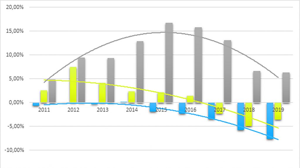
Source: [4]; MIWI Institute. Blue: Federal government (core and extra budgets); yellow: Federal states (core and extra budgets); grey: Municipalities (core and extra budgets).
2.2 Differentiation of the individual federal states
The overall analysis made is problematic in light of the fact that there are major fiscal policy differences between the individual federal states and their respective local communities. First of all, the consideration must be made as to which pattern these can be differentiated in the best possible way.
The German Economic Institute (IW Cologne) uses four groups of federal states for such analyses. Schleswig-Holstein and Lower Saxony form the northern group, Baden-Württemberg and Bavaria the southern group, the new federal states the east and Hesse, Rhineland-Palatinate and Saarland the western group. NRW is considered separately because of its size. [5; p.4]
The differences between the groups can be clearly seen in the level of debt. Table 2 demonstrates that the eastern group in particular is in a relatively good position in terms of debt. Only the state of Saxony-Anhalt is in a relatively poor position.
The states of Baden-Württemberg and Bavaria, as the southern group, historically have an almost good debt position, while both the western and northern groups are found at the bottom of the debt table.
Table 2. Per capita debt of German states and municipalities (as of 31 December 2020 in euros)
| Debts per capita as of December 31, 2020 in euros | Federal states | Municipalities | Sum | Rank – federal states | Rank – municipalities |
| Saxony | 1.244 | 575 | 1.819 | 13 | 13 |
| Bavaria | 1.359 | 1055 | 2414 | 12 | 8 |
| Baden-Wuerttemberg | 4.331 | 841 | 5172 | 11 | 11 |
| Mecklenburg-Western Pomerania | 5.247 | 1008 | 6255 | 10 | 10 |
| Brandenburg | 7.368 | 613 | 7981 | 7 | 12 |
| Thuringia | 7.363 | 1024 | 8387 | 8 | 9 |
| Hesse | 7.296 | 2258 | 9554 | 9 | 4 |
| Lower Saxony | 8.123 | 1698 | 9821 | 5 | 5 |
| Rhineland-Palatinate | 7.539 | 3182 | 10721 | 6 | 1 |
| Saxony-Anhalt | 9.705 | 1147 | 10852 | 4 | 7 |
| Schleswig Holstein | 11.002 | 1546 | 12548 | 2 | 6 |
| North Rhine-Westphalia | 9.957 | 2875 | 12832 | 3 | 3 |
| Saarland | 14.737 | 3158 | 17895 | 1 | 2 |
| Berlin | 16.307 | ||||
| Bremen | 57.823 | ||||
| Hamburg | 19.181 |
Source: [6]; MIWI Institute.
Table 2 also shows that in most cases the debt ranking of the federal state is related to the debt of the municipalities within that state. In Hesse, where the municipalities are financially significantly worse compared to the federal state, a “program to relieve Hessian municipalities of loans and to promote municipal investments was initiated. HESSENKASSE is the state’s offer to its municipalities to take 5 billion euros in cash loans from them, to organize debt reduction (…) and to provide state money itself to help pay off municipal debts.” [6]
In Rhineland-Palatinate, which currently has the highest per capita debt in relation to the municipalities, while the state itself has a place in the middle, a program for debt reduction for the municipalities was announced. [7] In Saarland, which is highly indebted both in terms of state and local government debt, the state has been taking over 1 billion euros in debt from cities and municipalities since 2020 as part of the Saarland Pact. [8]
Overall, a trend can be observed that the federal states are trying to let the municipalities participate in their more positive fiscal development.
2.3 Development of the federal states according to the level of indebtedness
The findings made in Section 2.2 relate to the data set at the end of 2020. Due to the heterogeneity of the federal states, it is interesting to see to what extent they have benefited from the boom.
For this reason, the development of the debts of the federal states including their municipalities and municipal associations in the period from 2010 to 2020 will now be considered.
A conceivable hypothesis would be that those federal states that already have had low debt in 2010 would have benefited more from the boom years since they generally have a better economic infrastructure, fewer internal transfer payments and lower debt service. On the other hand, an already low level of debt could reduce the motivation for further reductions and instead allow higher spending in other areas.
Table 3: Debt development of the federal states, including their municipalities (2010-2020, in euros per capita and percent)
| Rank | Federal state | 2020 | 2010 | Relative change |
| 13 | Saxony | 1819 | 2432 | 25,21 |
| 12 | Bavaria | 2314 | 3451 | 30,05 |
| 11 | Baden-Wuerttemberg | 5172 | 6044 | 14,43 |
| 10 | Mecklenburg-Western Pomerania | 6255 | 7426 | 15,77 |
| 7 | Brandenburg | 7981 | 8788 | 9,18 |
| 8 | Thuringia | 8387 | 8401 | 0,17 |
| 9 | Hesse | 9554 | 8544 | -11,82 |
| 5 | Lower Saxony | 9821 | 8448 | -16,26 |
| 6 | Rhineland-Palatinate | 10721 | 10316 | -3,93 |
| 4 | Saxony-Anhalt | 10852 | 10340 | -4,95 |
| 2 | Schleswig Holstein | 12548 | 10861 | -15,53 |
| 3 | North Rhine-Westphalia | 12832 | 12283 | -4,47 |
| 1 | Saarland | 17895 | 14644 | -22,2 |
| 3 | Berlin | 16037 | 17831 | 8,55 |
| 2 | Bremen | 19181 | 14119 | -35,85 |
| 1 | Hamburg | 57823 | 27372 | -111,25 |
Source: [6]; MIWI Institute.
Table 3 very clearly demonstrates a connection between a low starting level of debt and a high level of debt reduction in the period examined.
In this way, the three front runners, Saxony, Bavaria and Baden-Württemberg, were able to achieve additional debt reduction of around 15-30%. The taillights Schleswig-Holstein, North Rhine-Westphalia and Saarland, on the other hand, had to continue to borrow in the range of around 5-23%.
The graphic illustration from Figure 2 also shows in its entirety that there is a very clear connection between the development of debt reduction and the starting level debt.
Intermediate result:
Within the federal states and their municipalities, there is an enormous debt reduction asymmetry in relation to the starting level of debt in 2010. The most indebted federal states were not able to achieve net debt reduction even in 10 years of increasing economic output. Those federal states with a low starting level of debt were able to further reduce their debt by more than 10%, in some cases even up to 30%.
Figure 2. Development of debt relief in the federal states, including their municipalities (2010-2019, in percent)
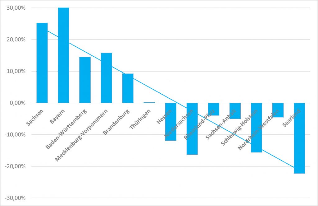
Source: [6]; MIWI Institute.
3. Not investing as the downside of debt
In the overall consideration in Section 2, the individual parameters have not yet been discussed, apart from the starting level of debt. In addition to the assumed positive development of income as a result of an economic upswing, there is a whole series of criteria that have had an influence on this development, especially on the government expenditure side.
With regard to the municipalities, for example, increases in income as a whole often could not have a positive effect because they were offset on the expenditure side, in particular by the increasing social expenditure. “The most obvious candidate for imbalances in many municipal budgets is social spending,” judges the IW Cologne. [5; p.4] There is also “a negative connection between social spending and investment spending (…). This illustrates how high social spending entails low investment.” [5; p.13]
With regard to public budgets, it is not an uncommon finding that, as a result of the overall development, investments are not made due to a lack of financial opportunities and are therefore seen as the downside of debt. [9; p. 26]
In its study on the differences in economic development in northern and southern Germany, the Institute for the World Economy (IfW Kiel) also examined the effects of economic development on public investment measures. The thesis was put forward that the different economic strengths of the northern and southern German federal states could also be linked to investment activity. [10, p. 15] In this context, one comes to the conclusion that the “richer South” spends a higher proportion of its government spending on investments in infrastructure. [10, p.19]. Thus there is also a connection between the investment ratio and debt reduction.
To put forward a hypothesis seems contradictory here. Because both investment measures and net debt relief initially constitute expenditure. To put it bluntly: Every euro that you repay cannot be invested. On the other hand, however, it could also be the case that participation in the economic upswing and lower social costs predominate to such an extent that both higher debt relief and an above-average investment ratio would be possible in a country comparison.
This is examined below. It should be noted that the data on the investment ratio is only available up to 2018, when the period up to 2020 was examined and therefore different assessment bases are available, which could lead to inaccuracies. Nevertheless, a trend can be derived.
Figure 3. Debt reduction vs. investment ratio of selected German federal states (2020 to 2010)
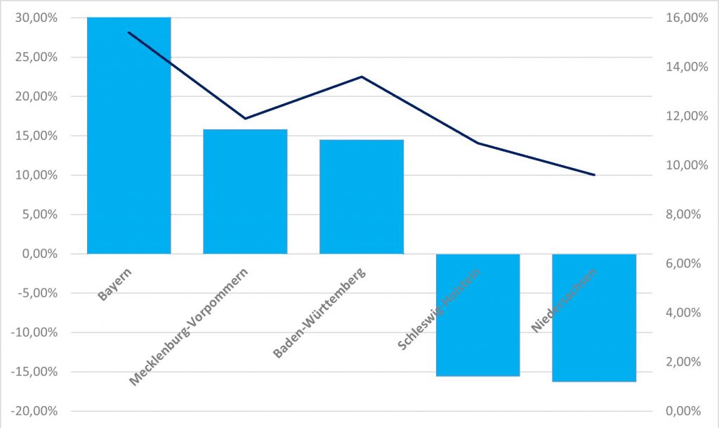
Source [6], [10], MIWI Institute. Light blue: Debt reduction (left axis, 2020 to 2010, percentage change); dark blue: investment ratio (right axis, 2010-2018, percentage change).
Intermediate result:
Figure 3 shows that there is a fundamentally positive relationship between debt reduction and the investment ratio. It appears that the economically more solid states are superior to the weaker states in terms of both the degree of debt reduction and the level of investment after a phase of economic upswing.
4. Prospects after 2020
With the start of the corona pandemic and currently as a result of the war in Ukraine, the signs of public finances have deteriorated significantly. [11, p.22] The resulting “disproportion in the long-term development of the state’s income and expenditure is reflected in the status quo scenario (…) of the generational balance in an implicit state debt (…).”
Expected increases in social and utility spending in the public sector, decreasing debt reduction from falling interest payments and no longer (to this extent) expected additional tax revenue suggest the thesis that debt reduction as in the 2010s is no longer possible in the foreseeable future. It is to be expected that this will particularly affect those federal states that were not able to achieve net debt reduction even during the 2010 boom period.
5. Results
In net terms, both the federal and state governments, in contrast to the local authorities, were on average able to use the 2010 boom years to deleverage their budgets. In some states, such as Hesse or Rhineland-Palatinate, there were and are initiatives to set up separate debt reduction programs for local authorities. As a result, this could result in an additional burden on the federal states.in the years to come.
The development is very heterogeneous within the individual federal states. Federal states with a low starting level of debt were once again able to deleverage disproportionately, while over a 10-year period more than half of the more heavily indebted federal states were not able to deleverage at all. There is a clear connection between the amount of net debt flow dynamics and the initial debt.
In addition, those federal states that were able to clear their debts significantly were also able to realize higher investment quotas and are therefore better positioned economically for the coming years.
6. Sources
[1] Destatis (2022). Bruttoinlandsprodukt (BIP) in Deutschland von 1991 bis 2021. URL: https://de.statista.com/statistik/daten/studie/1251/umfrage/entwicklung-des-bruttoinlandsprodukts-seit-dem-jahr-1991/
[2] Destatis (2022). Steuereinnahmen insgesamt in Deutschland von 2007 bis 2020. URL: https://de.statista.com/statistik/daten/studie/75423/umfrage/steuereinnahmen-in-deutschland-seit-1999/
[3] Destatis (2021). Staatsverschuldung: Höhe der Schulden des Öffentlichen Gesamthaushalts in Deutschland von 1991 bis 2020. URL: https://de.statista.com/statistik/daten/studie/633/umfrage/entwicklung-des-schuldenstands-der-oeffentlichen-haushalte-seit-1992
[4] Bundesfinanzministerium (2022). Schulden der öffentlichen Haushalte.
[5] Beznoska M., Kauder B. (2020). Schieflage der kommunalen Finanzen. IW Köln. URL: https://www.iwkoeln.de/studien/martin-beznoska-bjoern-kauder-schieflagen-der-kommunalen-finanzen.html
[6] Innenministerium Hessen (2021). Hessenkasse. URL: https://innen.hessen.de/Kommunales/Finanzen/Hessenkasse
[7] Finanzministerium Rheinland-Pfalz (2021). Anteilige Schuldenübernahme für rheinland-pfälzische Kommunen URL: https://fm.rlp.de/de/presse/detail/news/News/detail/anteilige-schuldenuebernahme-fuer-rheinland-pfaelzische-kommunen-gesetzentwurf-zur-verfassungsaenderung/
[8] Meves A.K. (2018). Saarland übernimmt 1 Milliarde Euro kommunaler Schulden. Der Neue Kämmerer. URL: https://www.derneuekaemmerer.de/haushalt/foederale-finanzbeziehungen/saarland-uebernimmt-1-milliarde-euro-kommunaler-schulden-9367/
[9] Junkernheinrich M. Micosatt G. (2017). Kommunalfinanzen in Rheinland-Pfalz Oder: Sind die Kommunen noch immer unterfinanziert? URL: https://landkreistag.rlp.de/homepage/downloads/finanzen-doppik/landesfinanzausgleichsgesetz/strukturelle-luecke.pdf?cid=mkk
[10] Schrader K., Laaser C.F. (2019). Unterschiede in der Wirtschaftsentwicklung im Norden und Süden Deutschlands. IfW Kiel. URL: https://www.ifw-kiel.de/de/publikationen/kieler-beitraege-zur-wirtschaftspolitik/unterschiede-in-der-wirtschaftsentwicklung-im-norden-und-sueden-deutschlands-0/
[11] Raffelhüschen B. et al. (2019. Die Generationenbilanz: Steigende Schulden, versäumte Reformen, apathische Politik. Stiftung Marktwirtschaft. URL: https://www.stiftung-marktwirtschaft.de/fileadmin/user_upload/Argumente/Argument_158_Update_Ehrbarer_Staat_2021_09.pdf