_ Alessandro Gasparotti, Policy Analyst, Department of Economics and Fiscal Policy, Centre for European Policy; Dr. Matthias Kullas, Head, Department of Economics and Fiscal Policy, Centre for European Policy. Freiburg, February 2019.*
Introduction
This year, the euro is celebrating its 20th birthday. From 1 January 1999, the euro could be used as bank money. The celebrations to mark this anniversary have, however, been muted. The reason for this is the still smouldering euro crisis. The euro crisis began at the end of 2009 in Greece and then engulfed numerous other eurozone countries. At its height in mid-2012, five of the then 17 eurozone countries – Greece, Ireland, Spain, Portugal and Cyprus – needed financial assistance: Via the specially created financial assistance funds – the EFSM, the EFSF and the ESM – as well as bilateral loans, Greece received EUR 261.9 billion, Ireland EUR 45 billion, Spain EUR 41.3 billion, Portugal EUR 50.3 billion and Cyprus EUR 6.3 billion. The situation only eased when, on 26 July 2012, the President of the European Central Bank (ECB), Mario Draghi, promised that the ECB would do everything within its mandate to uphold the currency union: “Within our mandate, the ECB is ready to do whatever it takes to preserve the euro.”1 Thus a breakup of the euro was just about averted.
Although Mario Draghi was able to reassure the capital market players with this promise, it did nothing to change the fundamental problems of the eurozone. In particular, the problem of the divergent competitiveness of the Eurozone countries remains unsolved. It arises from the fact that individual eurozone countries can no longer devalue their currency in order to remain internationally
competitive; a method commonly used before the euro was introduced. Since introduction of the euro, an erosion of international competitiveness leads to lower economic growth, a rise in unemployment and falling tax revenues. Greece and Italy in particular are currently experiencing major difficulties due to the fact that they are unable to devalue their currency.
In virtually every eurozone country, this trend has led to a discussion about the pros and cons of the single currency. Whilst the citizens of the troubled eurozone countries are lamenting low economic growth and high unemployment, other eurozone countries criticise Mario Draghi’s intervention and the fact that financial assistance makes them liable for the problem countries. Twenty years after its introduction, the euro is therefore more controversial than ever.
There is still a lack of reliable empirical data about which eurozone countries have gained from the introduction of the euro and which ones have lost out. Although there have been studies of whether the euro has promoted trade between eurozone countries,2 the results are not clear-cut. In addition, focussing on trade only throws light on a small aspect of the introduction of the euro. Disadvantages of introducing the euro arising from the fact that eurozone countries can no longer devalue their currencies, remain unaccounted for.
One meaningful indicator of whether, for individual eurozone countries, the euro has on balance led to a growth or a fall in prosperity, is the trend in gross domestic product per head of population (GDP per-capita). This therefore forms the basis of the following empirical examination in which the synthetic control method is used on selected eurozone countries to determine how per-capita GDP would have developed if they had not joined the eurozone. Comparing this with the actual trend in per-capita GDP indicates the impact that accession to the euro has had on prosperity. The analysis can only be carried out on eurozone countries in which there was a long gap between EU accession and introduction of the euro as this is the only way to ensure that the result of the analysis has not been distorted by accession to the EU and its internal market.
The analysis has therefore only been carried out in relation to Belgium, France, Germany, Italy, the Netherlands, Portugal and Spain. Although, as EU founding members, Luxembourg and Ireland also have sufficient distance between EU accession and introduction of the euro, the available data does not allow for a reliable conclusion to be drawn for these two countries.3
Methodology: The synthetic control method
The question we asked was: How high would the per-capita GDP of a specific eurozone country be if that country had not introduced the euro? This question is answered by means of the synthetic control method.4
The method allows the effects of a political measure – in this case the introduction of the euro – to be quantified on the basis of a specific measurement – in this case per-capita gross domestic product.5
Using the synthetic control method, the actual trend in per-capita GDP of a eurozone country can be compared with the hypothetical trend assuming that this country had not introduced the euro (counterfactual scenario).
The counterfactual scenario is generated by extrapolating the trend in per-capita GDP in other countries, which did not introduce the euro and which in previous years reported very similar economic trends to that of the eurozone country under consideration (control group). In order to obtain the best possible picture of the eurozone country, an algorithm is used to allocate a specific weighting to each country in the control group between 0% and 100%, the sum of the weightings being 100%. In this regard, the specific weightings are selected so that the weighted average of the trend in per-capita GDP of the control-group countries most closely resembles the trend in per-capita GDP of the eurozone country before it introduced the euro.6 The weightings are not based on considerations of plausibility but are determined by way of an econometric optimisation process.
The synthetic control method is far superior to other methods that only use a single non-euro-zone country for comparison, because the probability of obtaining a similar trend for the period prior to introduction of the euro and thus a realistic counterfactual scenario for the period after introduction of the euro, is much greater if, rather than just one country, a combination of several countries can be used each of which are allocated a different weighting.
Generating the weighted average of the control group is the core feature of the synthetic control method. It involves two steps. The first step is to select the countries worldwide that are to make up the control group for each individual eurozone country. They must fulfil the following conditions:
Firstly, only countries that have not been affected by major country-specific shocks during the whole of the relevant period – 1980 to 2017 – can be considered as such shocks may distort the results.
Secondly, they cannot be a eurozone country. Thirdly, the per-capita GDP of a control-group country in the years prior to introduction of the euro (pre-intervention period) must not diverge significantly from the GDP of the eurozone country under consideration (either up or down).7 This condition ensures that countries with a significantly higher or lower level of development do not distort the results for the counterfactual scenario.
The longer the pre-intervention period chosen, the greater the reliability of the results. We base our calculations on the period 1980 to 1996. Ending the period in 1996 may seem surprising since the euro exchange rate was not irrevocably established until 1 January 1999 – three years later. It may be assumed, or at least not ruled out, however, that market operators – due to the impending introduction of the euro – had already changed their behaviour prior to 1999.8
As a result of the third condition, the control groups for the various eurozone countries considered, are each made up of different countries. The control groups for each of the examined eurozone countries are set out in the Annex.
The second step is to determine a weighting from 0% to 100% for each country in a control group, using an econometric algorithm, so that the weighted average of the control group reproduces as accurately as possible the trend in per-capita GDP in the examined eurozone country before introduction of the euro. The greater the similarity between a country in the control and the examined eurozone country, prior to introduction of the euro, the higher its weighting will be. To obtain the weighting, firstly the trend in per-capita GDP (prices from 2010 in US-$9 ) in the control group countries is compared with that of the examined eurozone countries. Secondly, additional economic figures with a major influence on per-capita GDP, are taken into account. These are specifically the inflation rate, output from industry and the construction sector (as a % of GDP), fixed capital formation (as a % of GDP) and total exports and imports from goods and services (as a % of GDP). 10
When interpreting the results, the following must be considered: The synthetic control method implicitly assumes that no reforms were taken to increase per-capita GDP after introduction of the euro, either in the eurozone country under examination or in the countries in the relevant control group with a weighting of > 0, nor were any measures taken to reduce the per-capita GDP. In reality, this assumption is of course seldom true. This does not, however, invalidate the synthetic control method: Firstly, the results are so robust that minor reforms do not cast doubt upon them. Secondly, in the case of fundamental reforms, it depends how these were carried out. Where, for example, the examined eurozone country carried out a fundamental reform, after introduction of the euro, which increased per-capita GDP, but the countries in the control group did not, this may in principle result in an overestimation of the benefits of introduction of the euro. Experience has shown, however, that it was in fact the euro itself that prompted some eurozone countries to take reforms which in all likelihood they would not otherwise have carried out. In this case, the result is obviously not distorted by the reform.
Results summary on the effects of the introduction of the euro
For each of the examined eurozone countries, Table 1 indicates in euros how much higher or lower their per-capita GDP would have been, in 2017 (column 2) and overall (column 3), if they had not introduced the euro.
Tab. 1: Effects of the introduction of the euro on GDP in 2017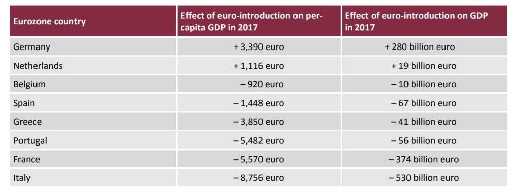
In 2017, out of the examined eurozone countries, only Germany and the Netherlands gained from the euro. In Germany, GDP went up by EUR 280 billion and per-capita GDP by EUR 3,390. Italy lost out most.
Without the euro, Italian GDP would have been higher by EUR 530 billion, which corresponds to EUR 8,756 per capita. In France, too, the euro has led to significant losses of prosperity of EUR 374 billion overall, which corresponds to EUR 5,570 per capita.
Table 2 shows the effects of the introduction of the euro on prosperity, per capita (column 2) and overall (column 3), for the entire period since the year of introduction – 1999 in all countries except Greece, for Greece 2001 – until 2017. The effects on prosperity are determined by adding the annual per-capita figures and multiplying the resulting amounts by the average national consumption rate11 of the relevant eurozone country in the pre-intervention period.12
Tab. 2: Cumulative effects of the introduction of the euro on prosperity 1999 to 2017
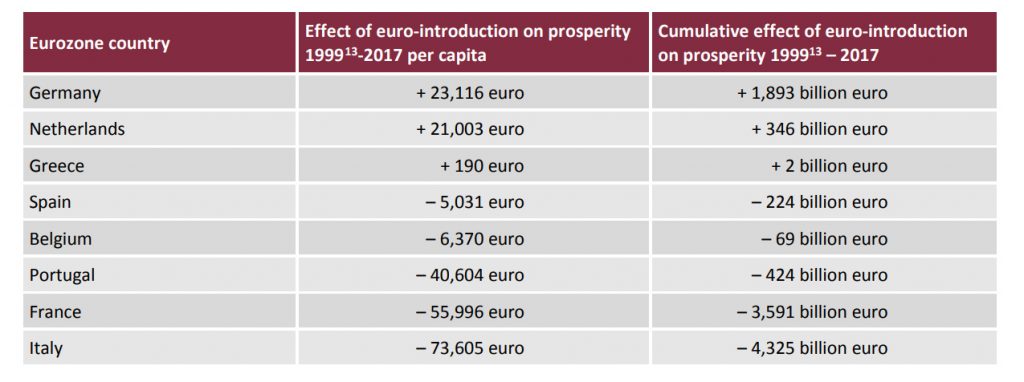
In Italy, therefore, the introduction of the euro led to a drop in prosperity of around EUR 74,000 per capita or EUR 4.3 trillion for the economy as a whole, over the period 1999 to 2017. For France, the loss amounts to almost EUR 56,000 per capita or EUR 3.6 trillion respectively. Germany achieved an increase in prosperity of EUR 23,000 per capita and EUR 1.9 trillion respectively.
The fact that the effects of the euro on prosperity in Greece are still just about positive is due to the fact that Greece gained hugely from the euro in the first few years after its introduction. This changed in 2011 after the bubble, created in previous years, burst in 2009. Since then, the euro has had a negative influence on Greek prosperity.
Notes:
- Speech by Mario Draghi, President of the European Central Bank, at the Global Investment Conference in London on 26 July 2012, online at: https://www.ecb.europa.eu/press/key/date/2012/html/sp120726.en.html, accessed on 15.01.2019.
- See e.g. Berger and Nitsch (2005) CesIfo Working Paper 1435, Bun and Klaassen (2007) Oxford Bulletin of Economics and Statistics, Faruqee (2004) IMF Working Paper 154, Rose and Stanley (2005) Journal of Economic Surveys or Baldwin (2006) ECB Working Paper 594.
- For details see Methodology.
- Abadie and Gardeazabal (2003) The American Economic Review, Abadie et al. (2010) Journal of the American Statistical Association and Abadie et al. (2015) American Journal of Political Science.
- The statistical package can be executed on MATLAB, STATA and R. We used STATA in our calculations. This package is available at: https://web.stanford.edu/~jhain/synthpage.html (last accessed on 15.01.2019).
- For an overview of the control-group countries and their weightings, see Annex.
- This condition for the selection of control-group countries was established by Puzzello and Gomis-Porqueras (2018). For details of this condition see Puzzello and Gomis-Porqueras (2018) European Economic Review.
- For Greece, which introduced the euro two years later, the pre-intervention period extends from 1980 to 1998.
- In order to display the results in euro – using the World Bank’s method – a $/EUR exchange rate of 1.324 is used.
- All data comes from the World Bank (http://data.worldbank.org/).
Source: https://www.cep.eu/
*Republished for research and educational purposes.